Find Maxima of Function using PSO Method || Numerical Example || ~xRay Pixy

Find the maximum value for the objective function using Particle Swarm Optimization Step-By-Step.

Video Chapters: Find the Maxima of Function using the PSO Method

00:00 Introduction

02:18 Objective

03:17 Maximization Problem

04:22 Particle Swarm Optimization Steps

05:22 Step 1 - Objective Function

05:30 Step 2 - Position and Velocity Initialization

06:00 Step 3 - Fitness Calculation

07:06 Step 4 - Update Personal Best

07:16 Step 5 - Update Global Best

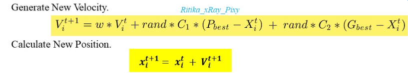
07:42 Step 6 - Position Update

10:34 Step 7 - Solution Boundary Checking

10:53 Step 8 - New Solution Evaluation

11:31 Step 9 - Update Personal Best

12:12 Step 10 - Update Global Best

13:24 Iteration 2 Start - Position Update

14:45 New Solution Boundary Checking

15:24 New Solution Fitness Calculation

15:48 Update Personal Best

16:32 Update Global Best

17:42 Conclusion

Problem: Find the Maxima of the function

$�(�)={�}^2+2�+11$$�(�)=�2+2�+11f(x)=x$

in the range -2<=x<=2 using PSO method. Use 4 particles (N = 4) with the initial
positions x1 = -1.5, x2 = 0.0, x3 = 0.5 and x4 =1.25. Show detailed computation 
for iteration 1. Assume w = 0.8 and C1 = C2 = 2.05.

Calculation for Iteration 01

Step 1: Define Objective Function

$�(�)={�}^2+2�+11$

Step 2: Initialize Position and Velocity for Each Particle (N = 1,2,3,4)

Initial Positions: x1 = -1.5, x2 = 0.0, x3 = 0.5, x4 = 1.25
Initial Velocities: v1 = v2 = v3 = v4 = 0
Weight Inertia (w) = 0.8
Acceleration Coefficients c1 = c2 = 2.05

Step 3: Evaluate Performance using Objective Function

f(x1) = -(-1.5)^2 + 2 (-1.5) + 11 = 5.75

f(x2) = -(0.0)^2 + 2(0.0) + 11 = 11

f(x3) = -(0.5)^2 + 2(0.5) + 11 = 11.75

f(x4) = -(1.25) ^2 + 2(1.25) + 11 = 11.93

Step 4: Update Personal Best Positions

Pbest(x1) = -1.5

Pbest(x2) = 0.0

Pbest(x3) = 0.5

Pbest(x4) = 1.25

Step 5: Update Global Best Position

Gbest = (x4) = 1.25

Step 6: Update the Velocity and Position for each Particle

Particle (x1) New Velocity

v1 = 0.8 * 0 + 0.3 * 2.05 * (-1.5 - (-1.5)) + 0.6 (2.05)*(1.25-(-1.5))

v1 = 3.3825

Particle (x1) New Position

x(1) = -1.5 + 3.3825= 1.88

Particle (x2) New Velocity

v2 = 0.8 * 0 + 0.2 * 2.05 * (0.0 - 0.0) + 0.6 * (2.05)*(1.25-0.0)

v2 = 1.537

Particle (x2) New Position

x(2) = 0.0 + 1.537  = 1.537

Particle (x3) New Velocity

v3 = 0.8 * 0 + 0.4 * 2.05 * (0.5 - 0.5) + 0.1 * (2.05)*(1.25-0.5))

v3 = 0.1537

Particle (x3) New Position

x(3) = 0.5 + 0.1537 = 0.6537

Particle (x4) New Velocity

v4 = 0.8 * 0 + 0.9 * 2.05 * (1.25 - 1.25) + 0.2 * (2.05)*(1.25-1.25))

v4 = 0

Particle (x4) New Position

x(4) = 1.25 - 0  = 1.25

Step 07: Ensure New Solutions are within range

Step 08: Evaluate New Solution Performance using Objective Function

f(x1) = -(1.88)^2 + 2 (1.88) + 11 = 11.23

f(x2) = -(1.53)^2 + 2(1.53) + 11 = 11.72

f(x3) = -(0.65)^2 + 2(0.65) + 11 = 11.87

f(x4) = -(1.25) ^2 + 2(1.25) + 11 = 11.9

Step 09: Update Personal Best Positions

Pbest(x1) = 1.88

Pbest(x2) = 1.53

Pbest(x3) = 0.65

Pbest(x4) = 1.25

Step 10: Update Global Best Position

Gbest = (x4) = 1.25        Check Fitness (Old_Gbest) > Fitness (New_Gbest)

Check (11.93) > (11.23)

            (11.93) > (11.72)

            (11.93) > (11.87)

            (11.93) > (11.93)

Step 11: Update Global Best Position

Gbest = (x4) = 1.25 

Step 12: Check Stopping Condition

Check (Current_itr <= Max_iter)

Repeat Steps from Step 6 to Step 11

For Iteration 01 Gbest Position = (x4) = 1.25  and Fitness = 11.93